1 Introduction to Machine Learning
S&DS 265 — Lecture 1
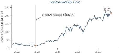
Artificial intelligence has taken off. In 2024 analysts called Nvidia’s developer conference “the Woodstock of AI”, and the company’s share price began its climb within weeks of the public launch of ChatGPT.
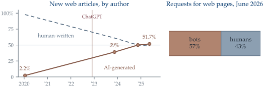
The change is not confined to a share price. Machine-written text has become a substantial part of what is published, and automated traffic a substantial part of what is requested.
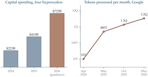
The resources behind this have grown on the same scale. The four largest cloud companies now spend more on data centres and accelerators each quarter than the entire industry spent in a year not long ago, and one provider’s monthly token volume rose from 10 trillion to 3.2 quadrillion in two years — a factor of roughly 300.
Two questions come before anything else. What is artificial intelligence? And since this is a course in machine learning, how are the two related?
1.1 Artificial Intelligence Is the Goal; Machine Learning Is How We Get There
Artificial intelligence names the goal: producing useful intelligent behaviour. Machine learning names the route that now dominates — fitting the rules to data instead of writing them down.
Hand-written rules were the older route. A programmer would study a problem, work out the logic, and state it explicitly: if the balance exceeds this threshold and the applicant has fewer than that many years of history, decline. The band of problems still handled that way keeps shrinking. On the problems this course cares about — prediction, perception, generation, and decision-making under uncertainty — almost everything is now learned.
That is why we will use AI and machine learning almost interchangeably, while keeping the distinction in view:
- Artificial intelligence — the goal of producing useful intelligent behaviour;
- Machine learning — constructing that behaviour by fitting models to data;
- Hand-written systems — rules stated directly by a person rather than learned.
1.2 Learning Means Predicting What We Have Not Seen
Machine learning looks for patterns in data we have observed, and turns them into a model that predicts well on data we have not.
observed data \longrightarrow a model that also works on new cases
The word doing the work is new. If a person’s income is already recorded in a database, returning it is retrieval, and no learning is involved. If income is unknown for a new person and has to be predicted from their education and seniority, the answer is not in the table at all. The model has to carry a pattern from the rows we have to a case we have never seen, and that transfer is the whole subject.
Four questions follow, and every topic in this course answers one of them:
- What data do we have?
- What kind of model do we allow?
- How do we build the model from the data?
- How do we tell whether it predicts well?
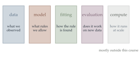
Compute is a fifth ingredient, and mostly a different subject. At frontier scale it dominates the engineering effort: distributed training across thousands of accelerators, memory hierarchies and activation checkpointing, quantization, communication schedules, interconnect bandwidth. We will meet compute where it changes the statistics — minibatches, stochastic gradients, why we stop early — and leave the systems engineering to courses built for it.
1.3 Three Learning Settings Differ in Where Feedback Comes From
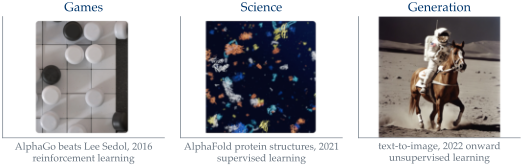
AlphaGo, AlphaFold, and a language model all use data, models, fitting, computation, and evaluation. What distinguishes them is the information available during learning.
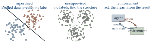
In supervised learning, the training data supply a target for each example and therefore contain pairs
\mathcal D_n=\{(x_i,y_i)\}_{i=1}^n.
The input x_i contains information available when a prediction is made; the target y_i records the desired outcome. If y_i is numerical, the problem is regression. If it is categorical, the problem is classification.
Examples include:
- predicting income from education and seniority;
- predicting whether a borrower defaults;
- mapping an amino-acid sequence to protein structure;
- classifying a handwritten digit from its pixels.
In unsupervised learning, the observations are x_1,\ldots,x_n with no externally supplied target. The method must therefore define another criterion for useful structure:
- PCA preserves variance or minimizes reconstruction error;
- clustering groups observations by a declared similarity;
- a mixture model explains data through latent components;
- an autoencoder reconstructs its input through a constrained representation;
- a generative model learns to produce new observations resembling the data.
The absence of labels does not mean the absence of an objective. It means the objective is constructed from the inputs rather than supplied as a separate response.
Self-supervision manufactures targets from unlabeled data. A language model hides or shifts part of a sequence and predicts it from the remaining context. The raw data have no human-provided label, but training can use supervised machinery because the sequence provides its own target:
\text{context tokens} \longrightarrow \text{next token}.
This is why language modeling can be described as unsupervised at the data level and supervised at the optimization level. The two statements answer different questions.
In reinforcement learning, action changes the data that will be observed. An agent sees a state, chooses an action, receives a consequence, and moves to a new state. There is no fixed dataset independent of the learner because the policy affects which future observations occur.
This creates a feedback loop:
\text{policy} \longrightarrow \text{actions} \longrightarrow \text{future data} \longrightarrow \text{updated policy}.
Evaluation must therefore account for the state distribution induced by the policy, not only performance on a static collection of past transitions.
Despite those differences, three questions recur:
- What structure does the model impose?
- How is the model fitted?
- What evidence would show that the fitted result worked?
The answer to the third question changes with the feedback process. A classifier can be evaluated on unseen labeled cases. A clustering needs stability or usefulness for a stated purpose. A policy must be evaluated under the consequences of its own actions.
A short history of AI. The ideas are far older than the excitement. Rosenblatt built the perceptron in 1958, a single layer that learned its weights from examples. Backpropagation was derived in the 1970s and brought to wide attention in 1986, which made many layers trainable at once. By 1989 LeCun’s convolutional networks were reading handwritten digits well enough for the postal service. Between those milestones sat two AI winters, in the mid-1970s and again around 1990, each following a stretch of confident promises that the available computers could not keep. The turn came in 2012, when AlexNet won the ImageNet competition by a margin large enough to end the argument. Three things had arrived together: labelled datasets of millions of images, GPUs fast enough to train on them, and architectures built to exploit both.
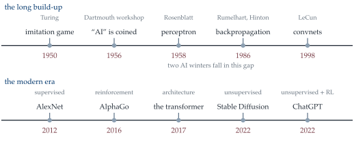
Two things follow from that timeline. Today’s systems took seventy years to arrive, and the methods along the way are still in service. Linear models, probability, dynamic programming, gradient methods, and neural networks all remain useful, because everything built later was built on them — which is why this course starts with the oldest of them.
1.4 Specifying a Prediction Problem
To make the workflow concrete, consider the 30 simulated people in the ISLP Income2 data. Each row records education, seniority, and income:
| person | education | seniority | income |
|---|---|---|---|
| 1 | 21.59 | 113.10 | 99.92 |
| 2 | 18.28 | 119.31 | 92.58 |
| 3 | 12.07 | 100.69 | 34.68 |
| \vdots | \vdots | \vdots | \vdots |
Education is measured in years and income in thousands of dollars. ISLP gives no unit for seniority anywhere, and its values run from 20 to 188, so they cannot be years either. The data are simulated. Knowing what a column measures is part of knowing what a fitted coefficient means, and no amount of modelling recovers it later.
Before fitting anything, read a row carefully. For person 1,
x_1= \begin{bmatrix} 21.59\\ 113.10 \end{bmatrix}, \qquad y_1=99.92.
The vector x_1 contains measurements that would be available when predicting; y_1 is the observed response. Calling the first two columns “features” and the last a “target” is a commitment about chronology and intended use.
The learning task concerns a new person, not one of the 30 people already recorded. Let
\mathcal D_n = \{(x_i,y_i)\}_{i=1}^n, \qquad x_i\in\mathbb R^d, \qquad y_i\in\mathbb R.
We seek a fitted rule \widehat f such that
\widehat y^\star = \widehat f(x^\star)
predicts the unknown income of a person with unseen features x^\star. Because the response is numerical, this is regression.
Examining income against education alone gives a curve in two dimensions. Using education and seniority together produces a surface in three dimensions. The same 30 people appear in both displays, but the second representation lets the model distinguish people with similar education and different seniority.
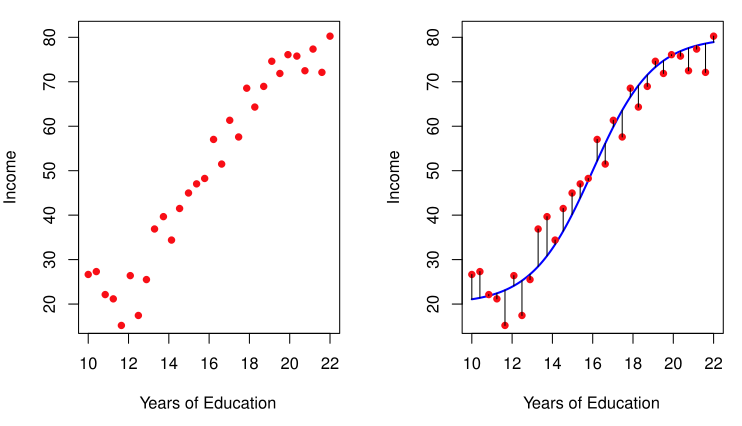
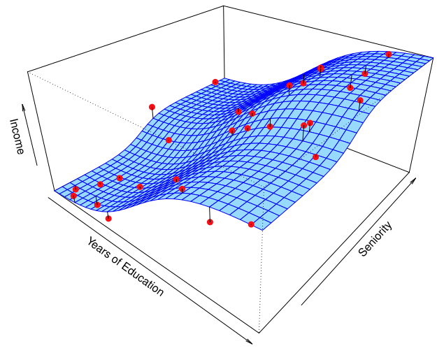
These are official ISLP Figures 2.2 and 2.3. The plots show an association, and they show where a straight line would misfit. Whether more education causes higher income is a different question, and this simulated data set has nothing to say about it.
The new person has no recorded income in the dataset. Prediction is possible only if the relationship seen among the 30 observed people remains informative for that person. Formally, we often imagine observed and future pairs drawn from a population distribution P:
(X_i,Y_i)\sim P.
Writing P once is an assumption, and a strong one: it says the world that produced the training rows is the world that will produce the next case. That assumption is what licenses using held-out performance as an estimate of future performance, and a shift in population, measurement, policy, or economic environment breaks it.
Some of the variation in income is explainable from education and seniority, and some of it is not. Splitting the response into those two pieces is what makes the distinction precise:
Y=m(X)+\varepsilon, \qquad m(x)=\mathbb E[Y\mid X=x], \qquad \mathbb E[\varepsilon\mid X]=0.
The conditional mean m(x) is the average response among all cases sharing the features x, and it is the best any rule could do knowing only X. Everything else lands in \varepsilon, where no choice of model reaches it, because X carries no information about it.
At a fixed x, any predictor f(x) has conditional squared risk
\begin{aligned} \mathbb E[(Y-f(x))^2\mid X=x] &= \mathbb E[ \{Y-m(x)+m(x)-f(x)\}^2 \mid X=x ]\\ &= \operatorname{Var}(Y\mid X=x) + \{m(x)-f(x)\}^2. \end{aligned} \tag{1.1}
The first term is irreducible error for predictors using X; even m(x) cannot predict new noise. The second is reducible error caused by using a rule different from the conditional mean. “Irreducible” is relative to the features and target: better measurements may move variation from the first term into the second.
1.5 Model, Loss, and Training Make Different Commitments
A model class declares which patterns are available. A one-feature linear family, for example, is
\mathcal F = \{f_\theta(x)=\theta_0+\theta_1x: \theta=(\theta_0,\theta_1)\in\mathbb R^2\}.
Training chooses one member of \mathcal F; it cannot leave the family. If the relevant relationship is strongly curved, perfect optimization of a line still produces a structurally inadequate model.
The phrase “all models are wrong, but some are useful” is not permission to ignore assumptions. It asks a sharper question: is the model wrong in a way that harms the intended prediction or decision?
A loss declares which mistakes matter and by how much. Squared loss charges the square of the error, so one large mistake costs more than several small ones:
\ell(y,\widehat y) = (y-\widehat y)^2.
It is symmetric in over- and underprediction and penalizes a two-unit residual four times as much as a one-unit residual. Those properties may be desirable, or they may misrepresent the application.
Parallel alternatives encode different priorities:
- absolute loss \lvert y-\widehat y\rvert grows linearly and is less dominated by large residuals;
- asymmetric loss can penalize underprediction more than overprediction;
- classification losses measure errors in scores or probabilities rather than numerical distance;
- decision-focused losses can represent downstream cost more directly.
The real-world goal and the training loss are related but not identical. A convenient objective must be defended as a proxy for the actual consequence.
What we want to control is population risk. For a rule f and future-data distribution P,
R(f) = \mathbb E_{(X,Y)\sim P} [\ell(Y,f(X))]
is the expected loss on a new case. We do not know P or R(f) exactly, so the training sample provides the observable empirical risk
\widehat R_n(f) = \frac1n\sum_{i=1}^n \ell(y_i,f(x_i)).
The population risk is unavailable, so the sample stands in for it, and the fitted rule is whichever member of the model class minimizes the observed average loss:
\widehat\theta \in \arg\min_{\theta\in\Theta} \widehat R_n(f_\theta). \tag{1.2}
This equation contains three prior decisions:
- the data decide which cases contribute;
- the model family decides which rules may compete;
- the loss decides how each error is scored.
Only after those choices does optimization begin.
Once the data, model, and loss have defined an objective surface over parameters, an optimizer searches that surface for a low value. Its answer is deliberately narrow: which available parameter setting scores well under the stated training objective?
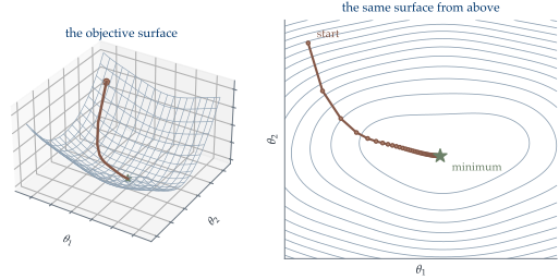
Optimization can fail because of poor scaling, initialization, stochastic noise, or nonconvexity. But even a global minimizer establishes only that the selected rule fits the training objective as well as possible within the chosen family. It does not show that:
- the target represents the actual goal;
- the sample represents future cases;
- the model family contains a useful relationship;
- the loss matches real costs;
- the selected rule generalizes.
During training, outcomes y_i are available and parameters change. During inference, the fitted parameters are held fixed and the model acts on a new x^\star whose outcome is unknown. For linear regression, the computational difference is small. For a transformer, the two stages differ radically in data access, memory, latency, and cost.
A campus dining-demand problem exposes the full specification:
| component | declared choice |
|---|---|
| case | one calendar day |
| features | weekday, forecast, events, recent demand |
| target | meals served from 11:30 to 1:30 |
| model | linear baseline or small regression tree |
| loss | absolute error if unit over- and under-preparation costs are similar |
| evidence | rolling evaluation on later unseen days |
Chronology belongs in the problem definition. Randomly interleaving adjacent dates between training and test sets can leak seasonality and operational changes. A technically valid split can be evidentially dishonest.
1.6 Flexibility Creates Both Opportunity and Overfitting
A larger family can represent more relationships. Polynomial regression illustrates this through nested model classes:
\mathcal F_k = \left\{ f(x)=\sum_{j=0}^k\theta_jx^j \right\}.
Every degree-1 polynomial is also available in degree 5 and degree 15 by setting higher coefficients to zero. Increasing k cannot make the minimum training loss worse. That monotonic fact is about optimization on observed rows, not prediction on new rows.
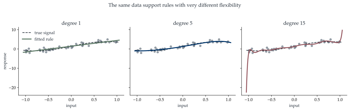
Flexibility need not be controlled by adding parameters. In K-nearest-neighbor classification, small K is flexible because each prediction depends on very few local observations. Large K averages over a wider region and produces a smoother boundary.
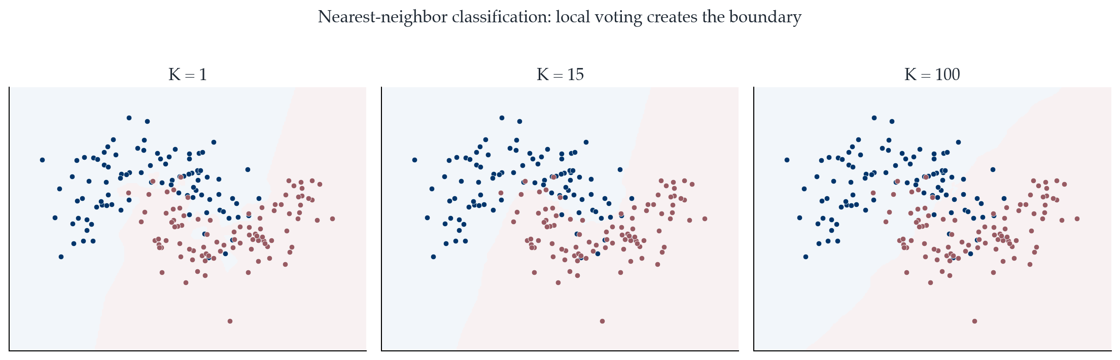
The polynomial degree and neighbor count move in opposite numerical directions—larger degree is more flexible, smaller K is more flexible. “Complexity” is a property of the function family, not a universal direction of a tuning parameter.
Training error is optimistic after fitting because the model was selected precisely for performing well on those observations. Reusing them to evaluate the selected rule ignores that selection. In the extreme, a one-neighbor classifier predicts every training label correctly, giving zero training error even when its boundary follows noise.
A fitted rule overfits when it captures sample-specific variation that does not repeat in relevant new data. The signature to look for is a gap: strong performance on the rows used for fitting, weak performance on genuinely unseen cases. Complexity alone is a poor diagnosis, since a complicated model that keeps its held-out accuracy has not overfitted anything.
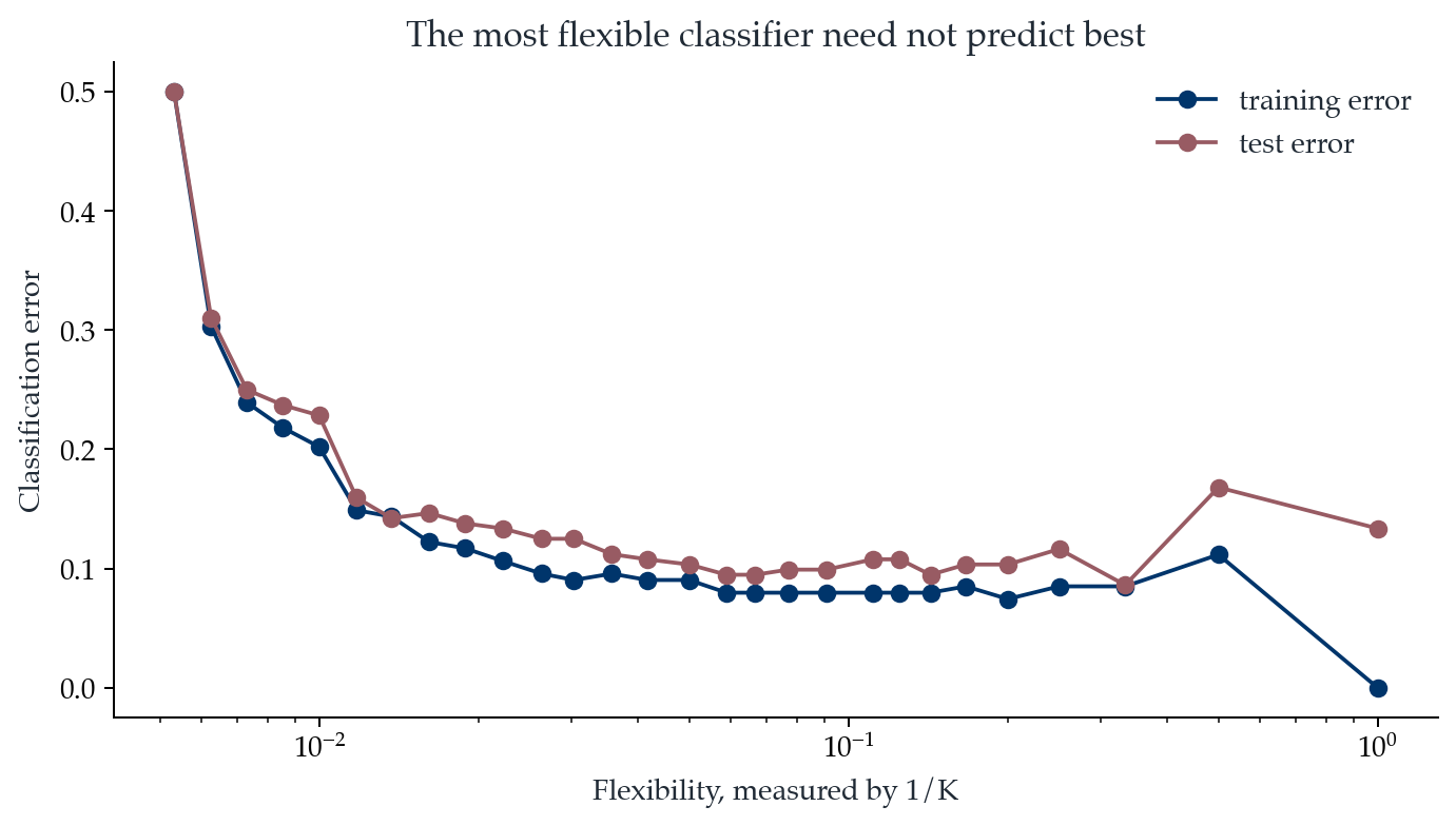
Bias and variance give a first explanation for that tradeoff. Imagine repeatedly drawing a training dataset \mathcal D and fitting \widehat f_{\mathcal D}. At a fixed x, suppose
Y=m(x)+\varepsilon, \qquad \mathbb E[\varepsilon\mid X=x]=0, \qquad \operatorname{Var}(\varepsilon\mid X=x)=\sigma^2.
Averaging over new outcomes and repeated training samples gives
\begin{aligned} \mathbb E_{\mathcal D,Y} [(Y-\widehat f_{\mathcal D}(x))^2\mid X=x] &= \sigma^2\\ &\quad+ \left( \mathbb E_{\mathcal D}[\widehat f_{\mathcal D}(x)] -m(x) \right)^2\\ &\quad+ \operatorname{Var}_{\mathcal D} (\widehat f_{\mathcal D}(x)). \end{aligned} \tag{1.3}
The three terms are:
- irreducible noise \sigma^2;
- squared bias, measuring systematic error in the average fitted rule;
- variance, measuring sensitivity to which training sample was observed.
Rigid families often have higher bias and lower variance. Highly flexible families can lower bias while increasing variance. This is a tendency, not a law governing every modern model, but it gives a precise first explanation for the U-shaped test curve.
Validation and test data therefore have different jobs:
- Fit parameters on the training set.
- Compare model families and tuning choices on validation data.
- Use the test set once for the final estimate of the entire selected procedure.
Repeatedly consulting test performance turns the test set into validation data. The final claim then needs a new untouched sample. Evidence is a resource that can be consumed by adaptive model selection.
1.7 What Counts as Evidence That a Model Works
A rule never generalizes “in the abstract.” It generalizes from a particular training process to particular unseen cases, and both halves have to be named before the claim means anything. For the Income example the future population might be people measured on the same variables by the same process. A change in the labour market, in how a variable is recorded, in who is eligible, or in how the sample was drawn can invalidate everything an earlier evaluation established.
The first question, then, is whether the evaluation imitates the intended use. What is one observational unit? When do the features become available, and is that before the moment a prediction is needed? Which future cases actually matter? A random split answers these only when the rows are exchangeable. Time series, repeated measurements on one patient, several images of the same subject, and geographically clustered observations all need a split that respects the grouping, because a random one puts near-duplicates on both sides of it and reports the resulting optimism as accuracy.
The second question is whether average loss is enough, and it rarely is. One number hides the comparison against a simple baseline, the uncertainty around itself, whether the residuals show a pattern the model missed, and whether some subgroup is served far worse than the mean suggests. It says nothing about behaviour under a plausible shift, about latency and memory, or about what the failures actually cost when they happen.
The third question comes earlier than either, at problem formulation, because the choices made there decide what the later numbers can reveal at all. Choosing the target decides what the system will optimize. Choosing the data decides whose experience is represented. Choosing the loss decides which mistakes matter. Choosing the evaluation decides which failures stay visible. An income model used for research, for lending, for marketing, and for public policy is the same arithmetic with four different sets of consequences; and where historical outcomes record unequal access or past decisions, predicting them accurately reproduces the process that produced them.
Keeping those layers apart is what the rest of this book does, one layer at a time:
- Question — what must be predicted, represented, generated, or decided for an unseen case?
- Evidence — which observations exist, and how were they produced?
- Structure — what relationship is assumed to persist?
- Model — which candidate rules express that assumption?
- Objective — what counts as success during fitting?
- Computation — how is a fitted solution constructed?
- Inference — how is the fitted solution used on a new case?
- Evaluation — what observation would support, or falsify, the claim that it works?
Optimization is one link in that chain, which is why a small training loss can sit quite happily alongside a broken system. The model may predict the wrong target, the labels may be noisy, the split may leak, the population may have moved, the loss may ignore a cost that matters in one direction more than the other, the optimizer may have landed somewhere brittle, or the average may conceal a failure nobody would accept. The value of the chain is that it makes debugging constructive: when something is wrong, the useful move is to find which link failed.
1.8 Summary
Machine learning applies where a rule cannot be stated explicitly. A problem that admits a specification is programmed. Learning addresses the remainder, where the mapping from input to answer is known only through examples of it.
The three settings differ in the source of their feedback. Supervised learning observes the answer, unsupervised learning observes none, and reinforcement learning observes a consequence of having acted. The source decides what evidence of success can be collected at all.
A prediction problem is specified before it is computed. The observational unit, the role of each measurement, the units of record, and above all the identity of the unseen case must be fixed in advance. Predicting the income of a new individual is a different problem from retrieving the income of a recorded one, and fitting cannot repair a confusion between the two.
Model, loss, and training are three separate commitments. The model class restricts what can be expressed, the loss defines what counts as a good answer, and training is the search. Each fails independently, which is why each is named separately.
Flexibility carries a cost. A richer class expresses more, and it can also fit the sample in place of the population. The bias–variance decomposition names that trade without resolving it.
A small empirical risk is weak evidence. A global minimizer of the empirical risk may still carry large population risk, so evidence has to come from data the fit never touched. That is what the train/validation/test chronology is for.
Every object introduced here leaned on mathematics before that mathematics was developed: one case became a vector, a dataset became a matrix, prediction became a function, loss became a number, fitting became optimization, and uncertainty became a distribution.
Lecture 2 develops those objects carefully, so that dimensions, geometry, derivatives, probability, and computation graphs become tools you can use to check every step of the workflow.