2 Mathematical Language for Machine Learning
S&DS 265 — Lecture 2
This chapter reviews the mathematical background the rest of the course relies on. We cover vectors, norms, inner products, and hyperplanes; symmetric matrices, eigenvalues, and the singular value decomposition; gradients, Hessians, and the local shape of a loss surface; computation graphs and automatic differentiation; and probability, conditioning, and the multivariate Gaussian.
2.1 Vectors Turn One Case into Geometry
One case becomes one ordered vector. Consider a credit-card customer described by balance and income:
x= \begin{bmatrix} 729.53\\ 44{,}361.63 \end{bmatrix} \in\mathbb R^2.
The vector is not an anonymous list. Coordinate 1 means balance; coordinate 2 means income; both have units; their order must remain fixed wherever the model uses them. Geometry gives the same vector two complementary readings:
- as a point, it is one customer’s location in feature space;
- as an arrow, it is a displacement from the origin that can be added and scaled.
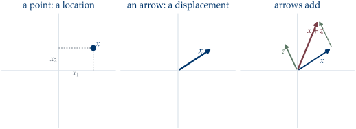
Linear combinations create a space of possibilities. Given vectors v_1,\ldots,v_k, their span is
\operatorname{span}\{v_1,\ldots,v_k\} = \left\{ \sum_{j=1}^k\alpha_jv_j:\alpha\in\mathbb R^k \right\}.
The span is a subspace: it contains the origin and is closed under addition and scalar multiplication. One nonzero vector spans a line; two independent vectors span a plane. The dimension is the number of independent directions, not the number of vectors used to describe them.
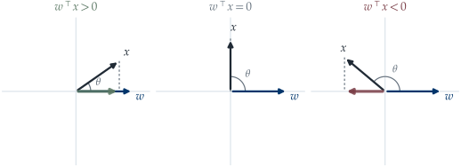
The inner product is both a score and an angle. For w,x\in\mathbb R^d,
w^\top x=\sum_{j=1}^dw_jx_j.
As a model computation, each feature contributes w_jx_j to one score. As geometry,
w^\top x =\lVert w\rVert_2\lVert x\rVert_2\cos\theta.
The score is positive when the vectors point partly together, zero when they are orthogonal, and negative when they point partly in opposite directions.
Orthonormal bases make coordinates into projections. Vectors u_1,\ldots,u_k are orthonormal when
u_i^\top u_j= \begin{cases} 1,&i=j,\\ 0,&i\ne j. \end{cases}
If u_1,\ldots,u_d form an orthonormal basis of \mathbb R^d, then every vector has the reconstruction
x=\sum_{j=1}^d(u_j^\top x)u_j.
The coefficient u_j^\top x is obtained by an inner product rather than by solving a new linear system. This simple fact powers orthogonal projection, eigendecomposition, the SVD, and PCA.
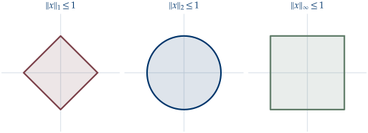
Length is not a single notion. A norm is any rule for measuring size that behaves sensibly under scaling and addition, and the family below is indexed by one exponent. For p\ge1, For p\ge1,
\lVert x\rVert_p = \left(\sum_j|x_j|^p\right)^{1/p}.
The exponent p decides how the coordinates are aggregated, and three choices cover nearly all use in this course:
\lVert x\rVert_1=\sum_j|x_j|, \qquad \lVert x\rVert_2=\sqrt{\sum_jx_j^2}, \qquad \lVert x\rVert_\infty=\max_j|x_j|.
For x=(3,-4), these values are 7, 5, and 4. The formulas do more than return different numbers: their unit balls have different geometry.
Scale determines the geometry the model sees. In the customer vector, raw income is numerically much larger than balance. A Euclidean distance on the raw coordinates will therefore be dominated by income. Standardization is not cosmetic: it changes which observations count as nearby and how strongly a penalty treats different coefficients.
A linear score produces hyperplanes.
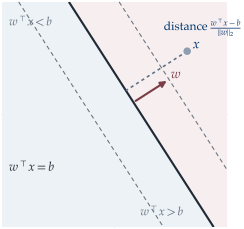
Definition 2.1 (Hyperplane) For w\in\mathbb R^d with w\ne0 and b\in\mathbb R, the hyperplane with normal w and offset b is the level set
H=\{x\in\mathbb R^d:w^\top x=b\}. \tag{2.1}
The vector w is normal to H in the following exact sense. If x,y\in H, then subtracting the two constraints gives w^\top(x-y)=b-b=0, so w is orthogonal to every direction lying inside the plane. Moving within H therefore leaves the score w^\top x unchanged, and w points in the direction that increases it fastest.
The distance from a point to H is now a short calculation, and it is worth doing carefully because the same quantity reappears as the margin in Lecture 9.
Proposition 2.1 (Signed distance to a hyperplane) For any x\in\mathbb R^d,
\operatorname{signed\ distance}(x,H) = \frac{w^\top x-b}{\lVert w\rVert_2}. \tag{2.2}
Its absolute value is the Euclidean distance from x to H, and its sign records which side of H the point lies on.
Proof. The closest point of H to x is reached by moving from x along the normal direction, since any component of the movement parallel to H only adds length without changing the constraint. Write that movement as
x^\star=x-\alpha w,
for a scalar \alpha to be determined. Requiring x^\star\in H means w^\top x^\star=b, and expanding the left-hand side gives
w^\top x^\star = w^\top x-\alpha\,w^\top w = w^\top x-\alpha\lVert w\rVert_2^2 = b,
where the middle equality uses w^\top w=\lVert w\rVert_2^2. Solving for \alpha, which is legitimate because w\ne0 makes \lVert w\rVert_2^2>0,
\alpha=\frac{w^\top x-b}{\lVert w\rVert_2^2}.
The displacement from x to the plane is x-x^\star=\alpha w, whose length is |\alpha|\,\lVert w\rVert_2. Substituting \alpha and cancelling one factor of \lVert w\rVert_2 leaves |w^\top x-b|/\lVert w\rVert_2. Dropping the absolute value keeps the sign of w^\top x-b, which is positive exactly on the side of H that w points toward. \blacksquare
Two consequences are worth recording. Scaling (w,b) by any c>0 leaves both H and the signed distance unchanged, so the pair is only determined up to positive scale — which is why margin methods in Lecture 9 must fix the scale by a normalization. And when \lVert w\rVert_2=1, the score w^\top x-b is the signed distance, with no division needed.
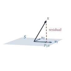
Projection finds the nearest explained component. For a unit vector u,
\operatorname{proj}_u(x) =(u^\top x)u =uu^\top x.
If a subspace S has orthonormal basis columns collected in U\in\mathbb R^{d\times k}, then
P_Sx=UU^\top x.
The residual x-P_Sx is orthogonal to every vector in S. For any z\in S, the Pythagorean identity gives
\lVert x-z\rVert_2^2 = \lVert x-P_Sx\rVert_2^2 + \lVert P_Sx-z\rVert_2^2.
The second term is nonnegative, so P_Sx is the closest point in S. This same argument will interpret fitted values in linear regression and reconstructions in PCA.
A matrix can be a table or a map. Stacking n cases as rows yields
X= \begin{bmatrix} x_1^\top\\ \vdots\\ x_n^\top \end{bmatrix} \in\mathbb R^{n\times d}.
As a table, rows are cases and columns are features. As a linear map, A\in\mathbb R^{m\times d} sends a vector in \mathbb R^d to one in \mathbb R^m. Thus Xw\in\mathbb R^n means one score per case, while XW\in\mathbb R^{n\times k} means k scores per case. The inner dimensions must agree algebraically; the summed-over dimensions must also mean the same thing.
2.2 Symmetric Matrices Reveal Directions and Scale
Quadratic forms turn directions into numbers. For a symmetric matrix A=A^\top,
q(x)=x^\top Ax =\sum_{i,j}A_{ij}x_ix_j.
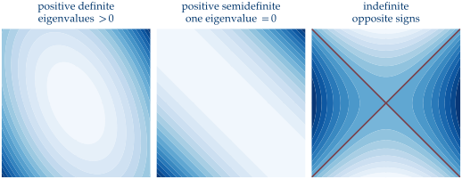
This form appears as a squared distance, a variance, and the curvature term of a Taylor approximation. We call A:
- positive semidefinite, written A\succeq0, if x^\top Ax\ge0 for every x;
- positive definite, written A\succ0, if x^\top Ax>0 for every nonzero x;
- indefinite if the form is positive in some directions and negative in others.
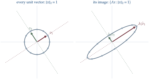
Most directions are rotated by a matrix as well as stretched. Eigenvectors are the exceptional ones that are only stretched, and that is exactly what the defining equation says: an eigenvector v\ne0 satisfiesctor v\ne0 satisfies
Av=\lambda v.
Along v, the map rescales without changing direction. For a real symmetric matrix, the spectral theorem gives an orthonormal eigenbasis:
A =V\Lambda V^\top =\sum_{j=1}^d\lambda_jv_jv_j^\top, \qquad V^\top V=I.
This decomposition does more than rewrite A; it diagonalizes every quadratic form built from it. Substituting A=\sum_j\lambda_jv_jv_j^\top into x^\top Ax and using x^\top v_jv_j^\top x=(v_j^\top x)^2,
x^\top Ax = \sum_{j=1}^d \lambda_j(v_j^\top x)^2. \tag{2.3}
Reading the identity. The cross terms are gone. In the eigenbasis the form is a weighted sum of squares, with the coefficient of the j-th square being exactly \lambda_j and the square itself being the squared component of x along v_j. Since every (v_j^\top x)^2\ge0, the sign of the whole expression is decided entirely by the signs of the eigenvalues.
That settles the classification immediately. The matrix is positive semidefinite exactly when every eigenvalue is nonnegative, because then every term is nonnegative for every x. Conversely a negative eigenvalue \lambda_k<0 supplies an explicit witness: taking x=v_k kills all the other terms and leaves x^\top Ax=\lambda_k<0. The same reading gives the geometry of Figure 2.6 — a zero eigenvalue is a direction along which the form is flat, which is the semidefinite case, and eigenvalues of both signs produce a saddle.
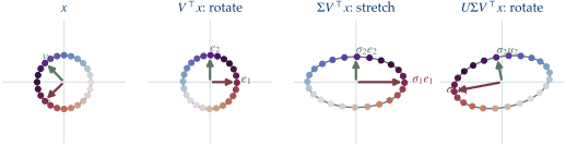
The SVD works for every matrix. A rectangular matrix A\in\mathbb R^{m\times d} with rank r has the thin singular value decomposition
\underbrace{A}_{m\times d} = \underbrace{U}_{m\times r} \underbrace{\Sigma}_{r\times r} \underbrace{V^\top}_{r\times d},
where U^\top U=V^\top V=I_r and
\Sigma=\operatorname{diag} (\sigma_1,\ldots,\sigma_r), \qquad \sigma_1\ge\cdots\ge\sigma_r>0. \tag{2.4}
Read from right to left, the map:
- rotates into right-singular-vector coordinates with V^\top;
- stretches those coordinates by the singular values;
- rotates into the output space with U.
Singular vectors are eigenvectors of two symmetric matrices. From Equation 2.4,
A^\top A =V\Sigma^2V^\top, \qquad AA^\top =U\Sigma^2U^\top.
Thus the right singular vectors are eigenvectors of A^\top A, the left singular vectors are eigenvectors of AA^\top, and the corresponding eigenvalues are \sigma_j^2. The SVD is not separate from eigendecomposition; it extends the same directional idea to maps between spaces of different dimensions.
Matrix norms summarize size, and the two that matter here answer different questions. The Frobenius norm treats the matrix as a long vector and measures its total energy,
\lVert A\rVert_F = \sqrt{\sum_{i,j}A_{ij}^2} = \sqrt{\sum_j\sigma_j^2},
where the second equality is the singular value decomposition read as a statement about energy: an orthogonal change of basis on either side leaves every entrywise sum of squares unchanged, so all of the matrix’s energy is accounted for by its singular values. The operator norm instead measures the worst-case stretch the matrix can apply to a unit vector,
\lVert A\rVert_{\mathrm{op}} = \max_{\lVert x\rVert_2=1}\lVert Ax\rVert_2 = \sigma_1,
and the maximum is attained at the top right singular vector, which is what makes it equal to the largest singular value \sigma_1 rather than some combination of them.
When the two norms disagree. Since \sigma_1^2\le\sum_j\sigma_j^2\le r\,\sigma_1^2 for a rank-r matrix, the two norms agree to within \sqrt r, so they can differ substantially for a wide matrix with many comparable singular values. The Frobenius norm is the one that appears in ridge penalties and reconstruction errors, because those objectives care about total deviation; the operator norm is the one that appears in stability arguments, because it bounds how far a perturbation can travel through a linear map.
The Frobenius norm treats the matrix as one long vector and is natural for total approximation error. The operator norm asks for the largest amplification of any unit direction.
Low rank means only a few stretches matter. Truncating the SVD after k<r terms gives
A_k = \sum_{j=1}^k\sigma_ju_jv_j^\top.
The Eckart–Young theorem says A_k is a closest rank-k approximation to A in both Frobenius and operator norm, with errors
\lVert A-A_k\rVert_F^2 =\sum_{j>k}\sigma_j^2, \qquad \lVert A-A_k\rVert_{\mathrm{op}} =\sigma_{k+1}.
Lecture 14 will turn this algebra into PCA and reconstruction.
Covariance is automatically PSD. For centered data X\in\mathbb R^{n\times d}, define
S=\frac1nX^\top X.
The covariance matrix is positive semidefinite, and the spectral reading above says why. For any direction w,
w^\top Sw = \frac1n w^\top X^\top Xw = \frac1n\lVert Xw\rVert_2^2 \ge0. \tag{2.5}
This number is the empirical variance of the scores Xw. Variance cannot be negative, so every covariance matrix is PSD. Its eigenvectors identify directions of spread, connecting probability, spectral algebra, and PCA.
2.3 Gradients and Curvature Describe Local Change
A derivative is a local linear model. For L:\mathbb R\to\mathbb R,
L(\theta+\Delta) = L(\theta)+L'(\theta)\Delta+o(|\Delta|).
The derivative is the slope of the best local straight-line approximation. Training uses it in exactly this sense: it predicts how a small parameter change alters the objective.
The gradient extends that approximation from one parameter to many. Each partial derivative \partial L/\partial\theta_j answers a one-dimensional question — how does the loss respond if I move coordinate j and hold the rest fixed? — and the gradient is the vector that collects all d answers:
\nabla L(\theta) = \begin{bmatrix} \partial L/\partial\theta_1\\ \vdots\\ \partial L/\partial\theta_d \end{bmatrix} \in\mathbb R^d .
Stacking the coordinatewise answers is more than bookkeeping, because it lets us predict the effect of moving in any direction, not only along the axes. For a displacement \Delta\in\mathbb R^d, taking the one-dimensional expansion along each coordinate and summing the contributions gives the first-order approximation
L(\theta+\Delta) \approx L(\theta)+\nabla L(\theta)^\top\Delta , \tag{2.6}
with an error that shrinks faster than \lVert\Delta\rVert_2 as the step shrinks. This is the statement training actually uses: the gradient is not primarily a list of slopes, it is the linear function that best predicts how the loss responds to a small move.
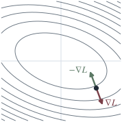
The change is an inner product, so the geometry from the first section applies. For a step of fixed length \lVert\Delta\rVert_2=\rho, Cauchy–Schwarz gives
\nabla L(\theta)^\top\Delta \ge -\rho\lVert\nabla L(\theta)\rVert_2,
Cauchy–Schwarz is an inequality about alignment: an inner product is bounded by the product of the lengths, with equality exactly when the two vectors are parallel. Here the lengths are fixed — \lVert\Delta\rVert_2=\rho by assumption — so the only freedom left is direction, and the bound is attained by pointing \Delta directly opposite the gradient:
\Delta = -\rho \frac{\nabla L(\theta)} {\lVert\nabla L(\theta)\rVert_2}.
The negative gradient is therefore the steepest local descent direction — but note the qualifier that made the argument work. “Steepest” was measured by the Euclidean length \lVert\Delta\rVert_2=\rho. Under a different notion of step size the extremal direction is different, which is exactly what the adaptive and second-order optimizers of Lecture 12 exploit.
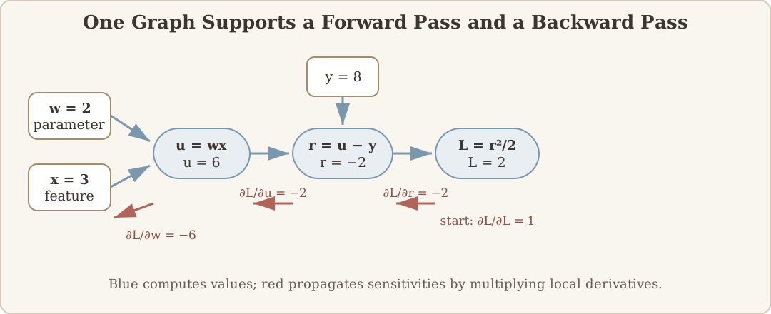
A simple loss shows the residual structure. For
\widehat y=\theta x, \qquad L(\theta)=\frac12(y-\theta x)^2,
the chain rule differentiates the outer square and then the inner linear function. The outer derivative of \tfrac12u^2 at u=y-\theta x is u, and the inner derivative of y-\theta x with respect to \theta is -x, so the two multiply to
\frac{dL}{d\theta} = (y-\theta x)\cdot(-x) = (\theta x-y)x .
The residual (\theta x-y) says whether the prediction is high or low; x says how strongly changing \theta moves it. At x=2, y=5, and \theta=1, the derivative is -6, so subtracting the gradient increases \theta and raises the prediction toward 5.
The Hessian describes how the gradient itself changes. The matrix of second derivatives is
\nabla^2L(\theta) = \left[ \frac{\partial^2L} {\partial\theta_i\partial\theta_j} \right]_{i,j}.
For a sufficiently smooth scalar loss, the Hessian is symmetric, and
L(\theta+\Delta) \approx L(\theta) + \nabla L(\theta)^\top\Delta + \frac12 \Delta^\top\nabla^2L(\theta)\Delta.
At a stationary point where \nabla L(\theta)=0:
- all positive Hessian eigenvalues describe a local bowl;
- mixed signs describe a saddle;
- a zero eigenvalue signals a locally flat direction requiring higher-order analysis;
- very unequal positive eigenvalues describe a long narrow valley.
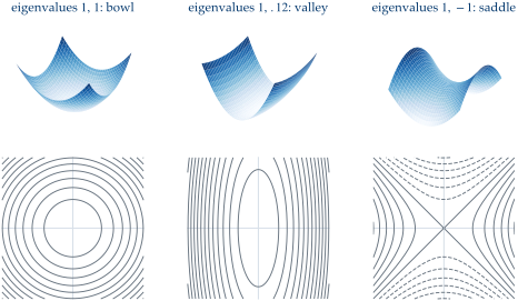
Local curvature and global convexity are different claims. A PSD Hessian at one point describes curvature there. If \nabla^2L(\theta)\succeq0 at every point in a convex domain, the function is convex. Then every local minimum is global. A single favorable Hessian cannot certify the entire surface.
Finite differences are a diagnostic, not a training method. A centered numerical derivative is
\frac{\partial L}{\partial\theta_j} \approx \frac{ L(\theta+\varepsilon e_j) - L(\theta-\varepsilon e_j) }{2\varepsilon}.
It needs two forward evaluations per coordinate, so it is too expensive for millions of parameters. It remains invaluable for checking a hand-derived or automatically computed gradient. If \varepsilon is too large, truncation error dominates; if it is too small, subtracting nearly equal floating-point values causes cancellation.
loss = lambda th, x=2.0, y=5.0: 0.5 * (y - th * x) ** 2
eps = 1e-5
numeric = (loss(1.0 + eps) - loss(1.0 - eps)) / (2 * eps)
analytic = (1.0 * 2.0 - 5.0) * 2.0
# numeric ≈ analytic ≈ -6
2.4 Computation Graphs Make the Chain Rule Scalable
A modern model is a composition, not one formula. Hand differentiation is exact but becomes unmanageable when an architecture changes. Finite differences are approximate and scale with the number of parameters. Automatic differentiation applies the ordinary chain rule to the operations that actually ran.
For a scalar loss and many parameters, reverse mode computes all parameter derivatives for a cost on the order of a small multiple of the forward computation. That output-to-input orientation is why backpropagation fits machine learning.
A graph records local dependencies. Consider a=wx, \qquad z=a+b, \qquad L=z^2.
The forward pass evaluates leaves to root and stores intermediate values. The reverse pass begins at the scalar loss and propagates sensitivities toward every parameter.
One numerical example makes every value visible. Let x=2, w=3, and b=-1. The forward pass gives
a=6, \qquad z=5, \qquad L=25.
The reverse pass starts from the trivial derivative of the loss with respect to itself, \partial L/\partial L=1, and walks the graph backwards. At each node it multiplies the sensitivity already accumulated at the node’s output by the derivative of that one local operation — which is the chain rule, applied one edge at a time.
Take the edges in order. The node L=z^2 contributes its own derivative 2z, so
\frac{\partial L}{\partial z}=2z=10 .
The node z=a+b has \partial z/\partial a=1, so passing through it leaves the incoming sensitivity untouched:
\frac{\partial L}{\partial a} = \underbrace{\frac{\partial L}{\partial z}}_{10} \cdot \underbrace{\frac{\partial z}{\partial a}}_{1} =10 .
This is the general rule for addition: a sum node copies its incoming sensitivity to each of its inputs unchanged. The node a=wx has \partial a/\partial w=x, so passing through it multiplies by the other factor:
\frac{\partial L}{\partial w} = \underbrace{\frac{\partial L}{\partial a}}_{10} \cdot \underbrace{\frac{\partial a}{\partial w}}_{x=2} =20 .
That is the general rule for multiplication: a product node routes the sensitivity to each input scaled by the input it was multiplied against, which is why the forward values must be stored before the backward pass can run.
The same sweep, continued along the two remaining edges, gives
\frac{\partial L}{\partial b}=10, \qquad \frac{\partial L}{\partial x}=10w=30 .
Note what the sweep did not do: it never formed a symbolic expression for L in terms of w, and it never re-ran the forward computation. Every parameter derivative came out of a single backward traversal reusing the stored forward values, which is exactly the cost claim made above.
Branches require addition. If an intermediate value affects the loss through several downstream paths, the chain rule adds those path contributions. For L=g_1(a)+g_2(a),
\frac{dL}{da} = \frac{dg_1}{da} + \frac{dg_2}{da}.
Backpropagation is the systematic accumulation of these products and sums. It is not a different calculus.
PyTorch builds the graph as code runs:
import torch

x = torch.tensor(2.0)
w = torch.tensor(3.0, requires_grad=True)
b = torch.tensor(-1.0, requires_grad=True)

a = w * x
z = a + b
loss = z ** 2
loss.backward()

w.grad, b.grad  # tensor(20.), tensor(10.)
The graph follows the executed operations, including ordinary Python control flow. Calling backward() differentiates the loss and fills leaf .grad fields; it does not update parameters.
Three rules prevent common autograd errors:
- Gradients accumulate into
.grad, so training code must clear them before the next backward pass. - Evaluation should use
torch.no_grad()when no derivative graph is needed. detach()returns a tensor cut from the current graph; use it deliberately, because detached computations cannot carry gradients back.
optimizer.zero_grad()
loss.backward()
optimizer.step()

model.eval()
with torch.no_grad():
    predictions = model(x_test)
Automatic does not mean self-validating. Autodiff gives the exact derivative of the program that ran. If the program uses the wrong loss, misaligns rows and outcomes, leaks test data, or broadcasts incompatible shapes, its derivatives can be perfectly correct for the wrong computation. A small hand derivation and finite-difference check remain part of trustworthy practice.
2.5 Probability and Gaussians Describe Uncertainty
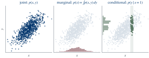
A joint distribution keeps variables together. For two random variables X and Y, the joint distribution p(x,y) describes how pairs occur. Marginalization removes one coordinate:
p(x)=\int p(x,y)\,dy, \qquad p(y)=\int p(x,y)\,dx,
with sums for discrete variables. Different joint distributions can share the same marginals, so marginalization discards dependence information.
Conditioning restricts attention to the cases where X=x and rescales so that what remains is again a distribution. For p(x)>0,
p(y\mid x) = \frac{p(x,y)}{p(x)}.
Conceptually, keep the cases with the observed x, then renormalize what remains into a distribution over y. Supervised learning asks about this object: what values of Y remain plausible after the features X=x are known?
The joint density can be factored two ways, conditioning on either variable, and equating the two factorizations is all Bayes’ rule is. Since. Since
p(x,y) =p(y\mid x)p(x) =p(x\mid y)p(y),
and carrying out that substitution we obtain
\underbrace{p(y\mid x)}_{\text{posterior}} = \frac{ \overbrace{p(x\mid y)}^{\text{likelihood}} \overbrace{p(y)}^{\text{prior}} }{ \underbrace{p(x)}_{\text{evidence}} }.
The denominator p(x)=\int p(x\mid y)p(y)\,dy normalizes the posterior. The likelihood is a function of the unknown y after x has been observed; it is not itself a posterior distribution.
Base rates remain visible after evidence. Suppose 5% of customers default. A warning fires for 80% of defaulters and 10% of non-defaulters. Then
P(\text{default}\mid\text{warning}) = \frac{0.80(0.05)} {0.80(0.05)+0.10(0.95)} \approx0.296.
The warning raises risk from 5% to about 30%, but it is not conclusive because false positives arise from the much larger non-default population. Lecture 7 will turn this logic into generative classification.
Expectation is a center; variance is squared spread. For a continuous random variable,
\mathbb E[X]=\int xp(x)\,dx, \qquad \operatorname{Var}(X) = \mathbb E[(X-\mathbb E[X])^2].
The standard deviation is a typical scale, not a bound. In several dimensions, covariance is
\operatorname{Cov}(X) = \mathbb E[ (X-\mathbb E[X]) (X-\mathbb E[X])^\top ].
The same computation applies to an arbitrary direction. For any w,
w^\top\operatorname{Cov}(X)w = \operatorname{Var}(w^\top X) \ge0,
which is the population version of Equation 2.5.
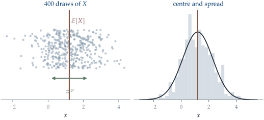
The univariate Gaussian turns distance into likelihood. If X\sim\mathcal N(\mu,\sigma^2),
p(x) = \frac1{\sqrt{2\pi\sigma^2}} \exp\left[ -\frac{(x-\mu)^2}{2\sigma^2} \right].
The mean translates the density; the variance controls its width. The exponent measures squared distance from \mu in units of \sigma.
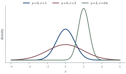
The choice of squared loss can be derived rather than assumed, by asking what noise model it corresponds to. Supposeuppose
Y\mid X=x \sim \mathcal N(f_\theta(x),\sigma^2).
Writing the same quantity for a single observation makes the pattern visible. For one observation,
-\log p(y\mid x,\theta) = \frac{(y-f_\theta(x))^2}{2\sigma^2} + \frac12\log(2\pi\sigma^2). \tag{2.7}
If \sigma^2 is fixed, maximizing conditional likelihood over \theta is equivalent to minimizing squared error. Lecture 3 will use that connection after first deriving least squares as an empirical-risk problem.
The multivariate Gaussian uses a quadratic distance. For x\in\mathbb R^d,
p(x) = \frac1{(2\pi)^{d/2}|\Sigma|^{1/2}} \exp\left[ -\frac12 (x-\mu)^\top\Sigma^{-1}(x-\mu) \right].
The exponent of the multivariate Gaussian is a quadratic form, so the spectral reading above applies directly to it. If
\Sigma=V\Lambda V^\top,
then its constant-density contours have axes v_j and lengths proportional to \sqrt{\lambda_j}. Off-diagonal covariance rotates the contours because knowing one coordinate changes what is plausible for another.
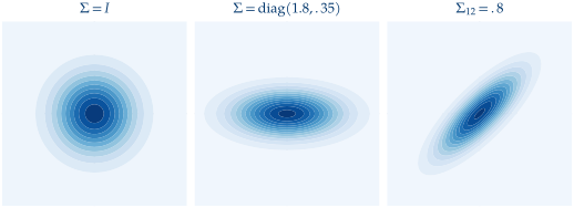
Linear maps preserve Gaussianity. This is the property that makes Gaussians so convenient: it lets us build any Gaussian we want out of the standard one, and it is what the reparameterization trick of Lecture 17 relies on.
Proposition 2.2 (Affine maps of a standard Gaussian) Let z\sim\mathcal N(0,I_d) and set x=Az+\mu for a matrix A\in\mathbb R^{d\times d} and a vector \mu\in\mathbb R^d. Then
x\sim\mathcal N(\mu,\,AA^\top).
Proof. There are two things to check: that the first two moments are as claimed, and that the distribution is still Gaussian at all.
Step 1: the mean. Expectation is linear, so it passes through the matrix and the shift separately:
\mathbb E[x]=\mathbb E[Az+\mu]=A\,\mathbb E[z]+\mu=A\cdot 0+\mu=\mu,
using \mathbb E[z]=0 for the standard Gaussian.
Step 2: the covariance. Since x-\mathbb E[x]=Az, the definition of covariance gives
\operatorname{Cov}(x)=\mathbb E\bigl[(Az)(Az)^\top\bigr]=\mathbb E\bigl[Azz^\top A^\top\bigr]=A\,\mathbb E[zz^\top]\,A^\top=AA^\top,
where the constant matrices A and A^\top come outside the expectation, and \mathbb E[zz^\top]=I_d because the coordinates of z are uncorrelated with unit variance.
Step 3: the family is preserved. Moments alone would not settle the shape of the distribution. What does is that every linear combination c^\top x=(A^\top c)^\top z+c^\top\mu is an affine function of a standard Gaussian vector, hence a scalar Gaussian; a random vector all of whose linear combinations are Gaussian is by definition multivariate Gaussian.
Together the three steps identify the distribution completely. \blacksquare
Reading the proposition as a sampler. Run backwards, it is a recipe. To sample from \mathcal N(\mu,\Sigma) for a given covariance \Sigma, find any A with AA^\top=\Sigma — the Cholesky factor, or V\Lambda^{1/2} from the eigendecomposition of the previous section — draw z\sim\mathcal N(0,I_d), and return Az+\mu. The randomness enters through z alone, and \mu and A are ordinary parameters that a gradient can flow through.
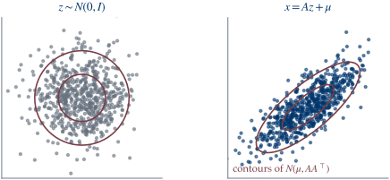
This closure property makes Gaussian models unusually tractable: linear transformations, marginals, and conditionals stay within the same family. It will support linear regression, discriminant analysis, mixtures, PCA-related latent models, and variational methods later in the course.
2.6 The Vocabulary Becomes a Verification Toolkit
Shape and meaning must be checked together. Let X\in\mathbb R^{n\times d} and w\in\mathbb R^d. The product Xw\in\mathbb R^n is legal because the inner dimensions agree. It is meaningful because rows are cases, columns are features, and w has one coefficient per feature.
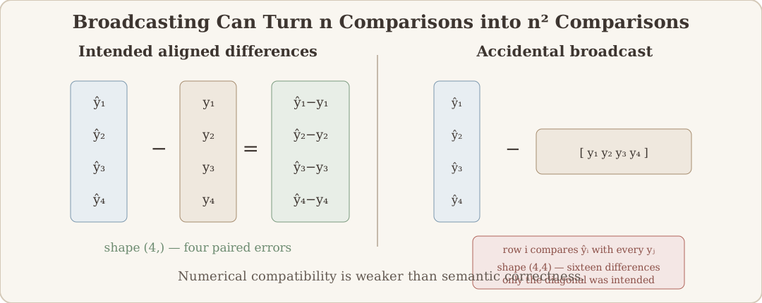
Broadcasting can defeat the second check. If predictions have shape (n,1) and outcomes have shape (n,), subtraction may produce an (n,n) matrix of all pairwise differences. The program runs and autodiff succeeds, but prediction i is no longer aligned with outcome i.
The objects introduced above recur throughout the course:
| object | question it answers | where it returns |
|---|---|---|
| inner product w^\top x | how do features combine into a score? | regression, logistic models, attention |
| hyperplane w^\top x=b | where does a linear score change decision? | classifiers and margins |
| projection UU^\top x | what part lies in a chosen subspace? | least squares and PCA |
| eigenvalues | which directions have positive, negative, or large effect? | curvature and covariance |
| singular values | which stretches dominate a general linear map? | conditioning and low rank |
| gradient | which local parameter change lowers loss fastest? | every differentiable training problem |
| Hessian | how does that local direction change with position? | convexity and optimization speed |
| conditional distribution p(y\mid x) | what remains uncertain after features are known? | prediction |
| covariance | which random directions vary together? | Gaussian models and PCA |
A reliable workflow begins before code:
- Name what each axis and symbol means.
- Write the intended input and output shapes.
- Calculate one small case by hand.
- State the assumption encoded by the operation.
- Check limiting or special cases.
- Compare an implementation with the hand result.
- Interpret the result in the original data problem.
2.7 Summary
A norm fixes what “close” means. The \ell_1, \ell_2, and \ell_\infty balls have different shapes, so they disagree about which points are neighbours. Rescaling a column changes that geometry.
A linear score defines a hyperplane. For the score w^\top x-b, the vector w is the normal direction and the signed distance to the boundary is (w^\top x-b)/\lVert w\rVert_2, the quantity that becomes the margin in Chapter 9.
A symmetric matrix scales along its eigenvectors. With S=Q\Lambda Q^\top, x^\top S x=\sum_j \lambda_j\,(q_j^\top x)^2, so definiteness is a statement about the \lambda_j, and a covariance matrix draws an ellipse.
Derivatives give the local linear and quadratic pictures. f(\beta+\delta)\approx f(\beta)+\nabla f(\beta)^\top\delta+\tfrac12\,\delta^\top\nabla^2f(\beta)\,\delta, the gradient setting the direction of steepest change and the Hessian the curvature around it.
Reverse mode differentiates in one traversal. A single backward pass over the operations that ran returns every \partial\mathcal L/\partial\theta_j at a small multiple of the forward cost. One scalar loss and many parameters is exactly the orientation machine learning needs.
Gaussians are closed under affine maps. If z\sim N(0,I) then \mu+Az\sim N(\mu,AA^\top), which builds every Gaussian from the standard one and makes the reparameterization of Chapter 17 possible.
Lecture 3 puts every one of these objects into a single complete regression problem: X is a design matrix, X\beta is a vector of predictions, squared loss is both an empirical risk and a Gaussian likelihood criterion, the gradient produces the normal equations, the Hessian proves convexity, and the fitted values are an orthogonal projection.
At that point the mathematics stops being a vocabulary list and becomes a connected explanation of what linear regression computes, and why.